Evaluating Object Proposals

[Update 05/19/2015: Please see our arXiv paper for an expanded version of the experiments described in this post: http://arxiv.org/abs/1502.05082.]

Object proposals have quickly become a popular pre-processing step for object detection. Some time ago I surveyed the state-of-the-art in generating object proposals, and the field has seen a lot of activity since that time! In fact, Larry Zitnick and I proposed the fast and quite effective Edge Boxes algorithm at ECCV 2014 (source code) (sorry for the self promotion).

So, How Good are Detection Proposals, Really? In their BMVC 2014 paper of the same name, Jan Hosang, Rodrigo Benenson and Bernt Schiele address this question, performing an apples-to-apples comparison of nearly all methods published to date. Highly recommended reading. While multiple evaluation metrics for object proposals have been proposed, ultimately object proposals are a pre-processing step for detection. In the BMVC paper, Jan and co-authors evaluated object proposals coupled with Deformable Part Models (DPMs). Surprisingly, some recent proposal methods which seemed quite promising based on recall plots resulted in rather poor detector performance.

So, I set out to see if there is a link between object proposal recall at various Intersection over Union (IoU) thresholds and detector average precision (AP). I asked the following: is proposal recall at a given IoU threshold (or thresholds) correlated with detector AP? Or do we need an alternate method for measure effectiveness of object proposals?

For the analysis I used the AP Pascal 2007 test scores for the DPM variant LM-LLDA. The AP numbers are obtained from Table 1 of Jan et al.’s BMVC paper. Recall values of each proposal method for each IoU threshold (at 1000 proposals) can be obtained from Figure 4b in Jan’s paper. However, while I used boxes provided by Jan I ran my own evaluation code (available here) to obtain the exact recall values (and the curves/numbers differ slightly from Figure 4b). Source code for reproducing these results can be found at the end of this post.

Here are the recall curves for 12 of the 14 methods evaluated by Jan et al. I excluded “Uniform” and “Superpixels” from the analysis since there AP is extremely low (under 20%). This is similar to Figure 4b from Jan’s paper except as mentioned I used my own evaluation code which differs slightly.

In the first experiment I computed the Pearson correlation coefficient between recall at various IoU values and AP. Here is the result: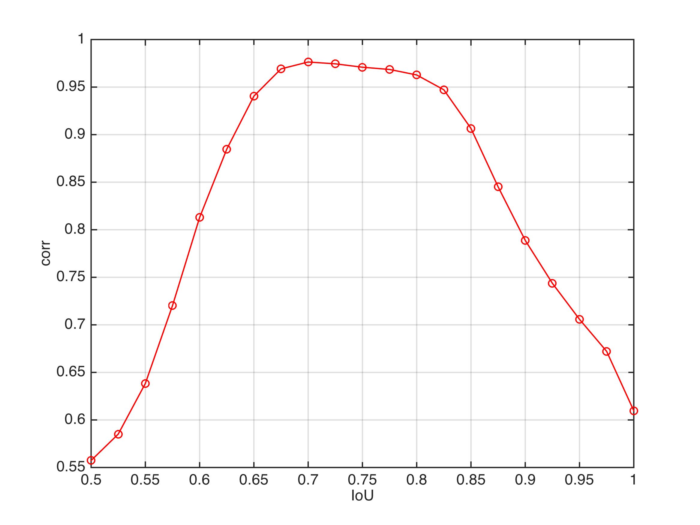For IoU values between 0.7 and 0.8 the correlation is quite high, reaching an r value of .976 at IoU of 0.7. What this means is that knowing recall of a proposal method at IoU value between 0.7 and 0.8 very strongly predicts AP for the proposals. Conversely, recall below about 0.6 or above 0.9 is only weakly predictive of detector performance.

Here is a scatter plot of recall at IoU of 0.7 versus AP for the 12 methods (a best fit line is shown):

As the high correlation coefficient suggests, there is a very strong linear relationship between recall at IoU=0.7 and AP.

I also analyzed correlation between recall across all IoU thresholds and AP by considering the area under the curve (AUC). However, correlation between AUC and AP is slightly weaker: r=0.9638. This makes sense as recall at low/high IoU values is not predictive of AP as discussed above. Instead, we can measure correlation between partial AUC (for a fixed threshold range) and AP. I found the optimal partial AUC for predicting AP is in the range of IoU thr of 0.625 to 0.850. The correlation in this case is r=0.984, meaning the partial AUC between these recall values predicts AP quite well. Here is the plot:

Overall, this is a fairly strong result. First, it implies that we should be optimizing proposals for recall at IoU threshold in the range of 0.625 to 0.850 (at least for DPMs). Note that his is despite the fact that in all the experiments AP was measured at a IoU of 0.5 for detector evaluation. Second, it means that we should be able to predict with reasonable reliability detector performance given recall in the given IoU range. One thing is clear: it is probably best to stop optimizing proposals for IoU of 0.5.

The main limitation of the analysis is that it is only for a single detector (DPM variant) on a single dataset (PASCAL 2007). It would be great to repeat for another detector, especially a modern detector based on convolutional neural networks such as Ross Girshick’s RCNN. Second, in the long term we definitely want to move toward having more accurate proposals. Presumably, as proposal accuracy improves, so will our ability to exploit the more accurate proposals.

---

I would like to thank Jan Hosang and Rodrigo Benenson for providing the output of all object proposal methods in a standardized format, and for Jan, Rodrigo and Ross Girshick for excellent discussions on the subject.

Matlab code for reproducing all results is below. Copying/pasting into Matlab should work. It is simple to swap in AP/recall for other detectors/datasets.

%% Recall matrix used for experiments nThresholds x nAlgorithms
R=[0.9196    0.8537 0.9197 0.8779 0.9116 0.8835 0.7724 0.8614 0.8107 0.8965 0.7737 0.4643
   0.8830 0.8339 0.9100 0.8566 0.8955 0.8669 0.7556 0.8407 0.7848 0.8831 0.7490 0.4391
   0.8276 0.8104 0.9013 0.8358 0.8769 0.8433 0.7409 0.8177 0.7564 0.8649 0.7218 0.4129
   0.7472 0.7875 0.8909 0.8125 0.8560 0.8108 0.7247 0.7924 0.7290 0.8438 0.6951 0.3881
   0.6483 0.7630 0.8801 0.7866 0.8349 0.7632 0.7089 0.7641 0.7026 0.8202 0.6643 0.3571
   0.5487 0.7360 0.8659 0.7575 0.8086 0.6973 0.6906 0.7322 0.6725 0.7957 0.6307 0.3216
   0.4450 0.7104 0.8488 0.7241 0.7811 0.6048 0.6727 0.7016 0.6425 0.7693 0.5936 0.2823
   0.3529 0.6818 0.8266 0.6884 0.7548 0.4953 0.6509 0.6699 0.6120 0.7388 0.5534 0.2423
   0.2743 0.6507 0.7941 0.6547 0.7241 0.3877 0.6263 0.6333 0.5737 0.7084 0.5076 0.2064
   0.2099 0.6178 0.7488 0.6160 0.6915 0.2879 0.6031 0.5964 0.5379 0.6740 0.4574 0.1711
   0.1587 0.5809 0.6855 0.5792 0.6560 0.2150 0.5724 0.5544 0.4961 0.6369 0.3985 0.1400
   0.1144 0.5396 0.6026 0.5342 0.6159 0.1578 0.5325 0.5106 0.4601 0.5913 0.3354 0.1109
   0.0850 0.4996 0.4982 0.4918 0.5713 0.1138 0.4599 0.4614 0.4175 0.5436 0.2685 0.0865
   0.0625 0.4490 0.3935 0.4417 0.5246 0.0812 0.3580 0.4154 0.3714 0.4931 0.1996 0.0662
   0.0456 0.3979 0.2886 0.3940 0.4728 0.0530 0.2369 0.3616 0.3256 0.4390 0.1368 0.0484
   0.0312 0.3430 0.1961 0.3424 0.4195 0.0328 0.1321 0.3020 0.2793 0.3791 0.0862 0.0352
   0.0225 0.2832 0.1258 0.2818 0.3542 0.0181 0.0648 0.2427 0.2245 0.3101 0.0480 0.0234
   0.0144 0.2149 0.0731 0.2135 0.2738 0.0086 0.0242 0.1786 0.1650 0.2363 0.0212 0.0141
   0.0091 0.1433 0.0358 0.1369 0.1834 0.0027 0.0051 0.1146 0.1022 0.1568 0.0076 0.0085
   0.0053 0.0621 0.0123 0.0623 0.0821 0.0004 0.0007 0.0498 0.0367 0.0696 0.0017 0.0046
   0.0001 0.0003 0.0003 0.0002 0.0002 0      0      0.0001 0.0001 0.0002 0      0 ];
save 'R' 'R';
%% define algorithm names, IoU thresholds, recall values and AP scores
nms={'Bing','CPMC','EdgeBoxes70','Endres','MCG','Objectness','Rahtu',...
  'RandPrim','Ranta2014','SelSearch','Gaussian','Slidingwindow'};
T=.5:.025:1; load R; %% see below for R matrix actually used in plots
AP=[21.8 29.9 31.8 31.2 32.4 25.0 29.6 30.5 30.7 31.7 27.3 20.7];
% plot correlation versus IoU and compute best threshold t
S=corrcoef([R' AP']); S=S(1:end-1,end); [s,t]=max(S);
figure(2); plot(T,S,'-or'); xlabel('IoU'); ylabel('corr'); grid on;
% plot AP versus recall at single best threshold t
figure(3); R1=R(t,:); plot(R1,AP,'dg'); grid on; text(R1+.015,AP,nms);
xlabel(sprintf('recall at IoU=%.3f',T(t))); axis([0 1 20 34])
title(sprintf('correlation=%.3f',s)); ylabel('AP'); hold on;
p=polyfit(R1,AP,1); line([0 1],[p(2),sum(p)],'Color',[1 1 1]/3); hold off
% compute correlation against optimal range of thrs(a:b)
n=length(T); S=zeros(n,n);
for a=1:n, for b=a:n, s=corrcoef(sum(R(a:b,:),1),AP); S(a,b)=s(2); end; end
[s,t]=max(S(:)); [a,b]=ind2sub([n n],t); R1=mean(R(a:b,:),1);
figure(4); plot(R1,AP,'dg'); grid on; text(R1+.015,AP,nms);
xlabel(sprintf('recall at IoU=%.3f-%.3f',T(a),T(b))); axis([0 1 20 34])
title(sprintf('correlation=%.3f',s)); ylabel('AP'); hold on;
p=polyfit(R1,AP,1); line([0 1],[p(2),sum(p)],'Color',[1 1 1]/3); hold off
% make figures nicer and save
for i=2:4, figure(i); hs=get(gca,{'title','xlabel','ylabel'});
  hs=[gca hs{:}]; set(hs,'FontSize',12); end
for i=2:4, figure(i); savefig(['corr' int2str(i)],'png'); end